Lecture 7: Formulas as a unifying domain for static analysis

General setup

Analysis domain based on formulas and main operations:

$A_0$ - set of all first-order formulas (or another set closed under propositional operations and quantifiers)
$A \subseteq A_0$ - subset of formulas that we use as our analysis domain, typically finite. If we used abstract interpretation framework, we would have $\gamma(F)=\{st \mid [\![F]\!]st = \mbox{true}\}$
$N : A_0 \to A$ - normalization function, ensuring that the result is in our domain, works as $\gamma$ but goes from formulas to formulas
- key requirement: the implication $F \rightarrow N(F)$ must be a valid formula ( $N$ produces a weaker formula)
$sp : A_0 \times \mbox{Com} \to A_0$ - computes strongest postcondition on formulas precisely, e.g. $sp(F(x),R(x,y)) = \exists x_1. F(x_1) \land R(x_1,x)$ . In some cases, we may want to eliminate the existential quantifier from the $sp$ formula, if for example $A_0$ allows the use of $\exists$ and $\forall$ , but $A$ doesn't. It really depends on what the analysis is about.

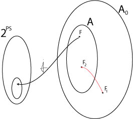
Note: $sp(F(x),R(x,y)) \in A_0$ and not in $A$ . We then should find a way to “put back” in $A$ what we obtain from $sp(F(x),R(x,y))$ . The figure below should help understanding the transformations. $F_1 \in A_0$ so we need the normalization function $N$ to push back $F_1$ in the set $A$ ( $N(F_1) = F_2$ ).

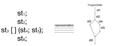
Control-flow graph is graph $(V,E)$ where $V$ are program points (between statements) and $E \subseteq V \times \mbox{Com} \times V$ are edges labelled with program commands.

Control Flow Analysis: Flow chart representation of a program. It is defined by some set of node ( $V$ ) and edges ( $E$ ).

Example:

As we are analyzing the program and we don't have any initial knowledge about the context we are starting in, we make our first assumption as general as possible.

The state of our analysis (set of computed facts) maps program points to formulas in $A_0$ , that is: $\mbox{fact} : V \to A_0$ .

Basic philosophy of the analysis: compute precise results whenever possible, then apply $N$ to fit it into $A_0$ .

Initial state: $\mbox{fact}_0(v)=\mbox{false}$ , except for initial program point $v_0$ , where $\mbox{fact}_0(v_0)=\mbox{true}$ . This can be different if we know something about the initial program state. For instance, when analyzing Java programs, we could use the fact that primitive data types are initialized to default values.

intuition: computing abstraction of the set of reachable states

Use the Update rule:

$\begin{equation*} \mbox{fact}_{i+1}(v) := N(\mbox{fact}_i(v) \vee \bigvee { sp(\mbox{fact}_i(u),c) \mid (u,c,v) \in E \} ) \end{equation*}$

to compute the impact of all incoming edges

For example, if we have a state $v$ reachable from two states $u_1$ and $u_2$ through the commands $c_1$ and $c_2$ respectively, we would have the following update rule for $\mbox{fact}(v)$ :

$\mbox{fact}_{i+1}(v) := N(\mbox{fact}_i(v) \vee sp(\mbox{fact}_i(u_1), c_1) \vee sp(\mbox{fact}_i(u_2), c_2))$

When we do an analysis we must consider two properties: Correctness (soundness) and Termination

Correctness (soundness): if for each program point $\mbox{fact}_{i+1}(v) \rightarrow \mbox{fact}_i(v)$ for all $v \in V$ , then the facts are true in all program executions and they correspond to loop invariant(s). For more information see correctness of formula propagation.

(If we stopped the analysis before this happens, then the result is not correct, it does not take into account all executions).

Note: To prove correctness for the guarded command [ ] (non-deterministic choice) we can choose any path we like, the only aspect that matters is fairness (in the choice).

Termination:

observe the sequence of formulas $\mbox{fact}_i(v)$ for $0 \leq i$
start from false, become weaker and weaker
require that there are no infinite ascending chains of weaker and weaker formulas

Analysis stops when $\forall v. \mbox{fact}_{i+1}(v) \rightarrow \mbox{fact}_i(v)$ . That is, no new states are generated by strongest postcondition (we have reached a fix point - formula not trivial).

Note: If you end up with a situation where $\exists$ a state $v$ for which $\mbox{fact}(v) = true$ , then the analysis gives no useful information about state $v$ . In this case, you may want to refine $A$ (and hence also change the function $N$ ). Sometimes, this can be done automatically.

Examples

Conjunctions of fixed predicates as analysis domain

(an example of Independent Attribute Analysis)

Definition of the domain

We have some predicates $P_1, P_2, ..., P_n$ and a set of formulas $A = \{P_{i1} \wedge ... \wedge P_{in} | 1 \le i_1 < ... < i_n \le n \}$ . Let us observe that $h(A) = n$ (the height of a tree representing a formula), and $|A| = 2^n$ (the number of possible formulas).

Normalization operator We define $N: A_0 \rightarrow A$ a normalization function (look at the General Setup at the top of the page for more details). We will look at two possible ways to construct it for our example.

First idea, computing abstract postcondition

We want to compute $N(sp(P_{i1} \wedge \ldots \wedge P_{in}, c))$ . In other words, we want to find some predicates that are true after conjunction of some predicates $P_i$ and command $c$ . We use the following construction:

$N(sp(P_{i1} \wedge \ldots \wedge P_{in}, c)) = \bigwedge \{ P_{ik} | sp(P_{i1} \wedge \ldots \wedge P_{in},c) \Rightarrow P_{ik} \}$

To understand why this is indeed a normalization, notice that even though $sp(\ldots,c) \subseteq A_0$ , we're computing a conjunction on predicates which are implied by the postconditions and therefore, this conjunction is also $\subseteq A$ .

(Alternatively, we can use weakest preconditions and write $N(sp(P_{i1} \wedge \ldots \wedge P_{in}, c)) = \bigwedge \{ P_{ik} | P_{i1} \wedge \ldots \wedge P_{in} \Rightarrow wp(P_{ik},c) \}$ .)

Second idea

$N: A_0 \rightarrow A$ is still a normalization function. We have $F \in A_0$ and we compute $N(F)$ such that $F \rightarrow N(F)$ is the strongest possible. If we are trying to find strongest precondition, then we would compute $\bigwedge \{ F_1 | F_1 \in A \wedge F \rightarrow F_1 \mbox{is valid}\}$

The intuition here is really to take all possible formulas in the simplified language which are implied by the formula to be normalized. To avoid weaker formulas, we take conjunction.

Note We may want to add the predicate $P_0 := false$ . Notice that if $false$ holds at any given point, then every property following will still hold. In other words, if you have some unreachable code in a program, then everything that follow will still be unreachable.

Example

Consider the following (embarrassingly simple) program:

y := 0
if(x > 0)
  y := 1
if(x > 0)
  y := -1

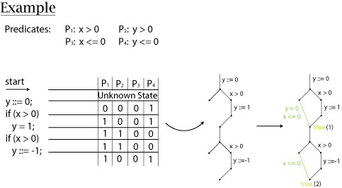
The following schema shows several things;

For all the predicates which can hold for this program (using $>$ , $\leq$ and omitting $false$ ), the table on the left shows which ones hold for a given program state. 1 means the predicate holds
The two graphs on the right are flow-graphs, where statements are represented as edges and states as vertices (nodes). On the second one, annotations in colours represent predicates (while the black text still mark statements).

Looking at the program, one should be able to state that at its end, $y$ will always be $\leq 0$ . However, the conclusion reached at the end of the analysis is $true$ , in other words, it tells us “the predicate $true$ is always true at the end of the program”. In yet other words, this tells us nothing interesting. Why the difference?

Someone looking at the program will certainly notice that the one place where $y$ is assigned to $1$ will have no effect on the final result. The reason is that the assignment is “canceled out” by another one which occurs for the same condition, $x > 0$ , and $x$ doesn't change in between.

The fact that we only used conjunctions is our analysis makes it path-insensitive. Intuitively, since we're only taking conjunctions, our normalization is too conservative and we will not be able to retain properties associated to certain paths. Path-sensitivity is often used as a measure of the precision of an analysis.

Disjunctions of conjunctions of predicates

(an example of Dependent Attribute Analysis)

As we just saw, our analysis domain turned out to be too restrictive. We may want to use a more extended one. Let's define a new set of formulas:

$A^+ = \{ \bigvee (P_{i1} \wedge ... \wedge P_{in}) | P_{ij} \in \{Q_1, ..., Q_n\}) \}$

The use of disjunctions allows us to write predicates about attributes for some particular paths. For this reason, this is called relational (or dependent) attribute analysis.

If we go back to our previous example, we could end up with a predicate at the final point which would look (at least partially) somehow like:

$(x > 0 \wedge y \leq 0) \vee (x \leq 0 \wedge y = 0)$

…where the first part represents the conclusions which can be made if the branches $x > 0$ were taken and the second the ones when they weren't. From there we'd find that $y \leq 0$ always holds. (Note that this is informal and was not done in class.)

The normalization function now looks like:

$N(sp(C_i \vee \ldots \vee C_n, C)) = N(sp(C_1, C) \vee sp(C_2,c) \vee \ldots \vee sp(C_n,c))$

$= N(sp(C_1,C)) \vee N(sp(C_2,c)) \vee \ldots \vee N(sp(C_n,c))$

While this construction is valid mathematically speaking and it allows us to express more properties on programs, we have a problem with the exponential growth of the size of $|A^+| = 2^{2^n}$ , and the height of the formulas $h(n) = 2^n$ . Consequently, we need some optimizations. For instance, we could do simplifications such as:

$(p \wedge q) \vee (\neg p \wedge q) \Rightarrow q$

For mode details, see the papers.

Note: There is a tradeoff between precision and efficiency.

Linear inequalities

(section not covered in class)

Example implementation: Parma Polyhedra Library and a paper about Parma. Geometric interpretation of linear equations.

Special cases:

constant propagation
interval analysis
octagon domain

Simple pointer analysis

All we have seen so far was about simple values. In complex programs we have runtime effects, e.g. pointer.

In fact, it can happen that two variables with different names (aliases) represent the same object (in memory). Take the following example:

C code: (x and y are two pointers already allocated)
*x = 3;
*y = 2;

The behavior of this program will strictly depend on the fact that pointers $x$ and $y$ are not pointing on the same memory address (so, in the code, there is no such statement $x = y$ ). The semantic that we have used since now doesn't allow to correctly handle those runtime effects.

Consider constant field propagation with

x = new Node();
y = new Node();
x.f = 1;
y.f = 2;

or with

y = x.next;
x.f = 1;
y.f = 2;

Allocation-site based analyses and logical representation of their abstract domains.